Chapter 3 Estatistica e R
A estatística descritiva busca fornecer uma descrição útil de um grande número de dados a partir de valores como média, mediana, variância, desvio padrão e quartis, frequencia de valores e moda, correlação e covariância.
Alguns essas medidas buscam descrever o dado em termos de seus valores, distribuição dos valores e correlação entre os dados.
3.1 Entendo os Dados e Estatística Descritiva
3.1.1 Exploração inicial dos dados
Significado ds dados, quantidade e linhas e colunas, tipos de dados.
Primeiras linhas de um dataframe
library(MASS)
help(Cars93)
## starting httpd help server ... donehead(Cars93)## Manufacturer Model Type Min.Price Price Max.Price MPG.city MPG.highway
## 1 Acura Integra Small 12.9 15.9 18.8 25 31
## 2 Acura Legend Midsize 29.2 33.9 38.7 18 25
## 3 Audi 90 Compact 25.9 29.1 32.3 20 26
## 4 Audi 100 Midsize 30.8 37.7 44.6 19 26
## 5 BMW 535i Midsize 23.7 30.0 36.2 22 30
## 6 Buick Century Midsize 14.2 15.7 17.3 22 31
## AirBags DriveTrain Cylinders EngineSize Horsepower RPM
## 1 None Front 4 1.8 140 6300
## 2 Driver & Passenger Front 6 3.2 200 5500
## 3 Driver only Front 6 2.8 172 5500
## 4 Driver & Passenger Front 6 2.8 172 5500
## 5 Driver only Rear 4 3.5 208 5700
## 6 Driver only Front 4 2.2 110 5200
## Rev.per.mile Man.trans.avail Fuel.tank.capacity Passengers Length Wheelbase
## 1 2890 Yes 13.2 5 177 102
## 2 2335 Yes 18.0 5 195 115
## 3 2280 Yes 16.9 5 180 102
## 4 2535 Yes 21.1 6 193 106
## 5 2545 Yes 21.1 4 186 109
## 6 2565 No 16.4 6 189 105
## Width Turn.circle Rear.seat.room Luggage.room Weight Origin Make
## 1 68 37 26.5 11 2705 non-USA Acura Integra
## 2 71 38 30.0 15 3560 non-USA Acura Legend
## 3 67 37 28.0 14 3375 non-USA Audi 90
## 4 70 37 31.0 17 3405 non-USA Audi 100
## 5 69 39 27.0 13 3640 non-USA BMW 535i
## 6 69 41 28.0 16 2880 USA Buick CenturyNúmero de linhas e colunas.
nrow(Cars93)## [1] 93ncol(Cars93)## [1] 27Examinando estrutura e tipos de dados.
class(Cars93)## [1] "data.frame"str(Cars93)## 'data.frame': 93 obs. of 27 variables:
## $ Manufacturer : Factor w/ 32 levels "Acura","Audi",..: 1 1 2 2 3 4 4 4 4 5 ...
## $ Model : Factor w/ 93 levels "100","190E","240",..: 49 56 9 1 6 24 54 74 73 35 ...
## $ Type : Factor w/ 6 levels "Compact","Large",..: 4 3 1 3 3 3 2 2 3 2 ...
## $ Min.Price : num 12.9 29.2 25.9 30.8 23.7 14.2 19.9 22.6 26.3 33 ...
## $ Price : num 15.9 33.9 29.1 37.7 30 15.7 20.8 23.7 26.3 34.7 ...
## $ Max.Price : num 18.8 38.7 32.3 44.6 36.2 17.3 21.7 24.9 26.3 36.3 ...
## $ MPG.city : int 25 18 20 19 22 22 19 16 19 16 ...
## $ MPG.highway : int 31 25 26 26 30 31 28 25 27 25 ...
## $ AirBags : Factor w/ 3 levels "Driver & Passenger",..: 3 1 2 1 2 2 2 2 2 2 ...
## $ DriveTrain : Factor w/ 3 levels "4WD","Front",..: 2 2 2 2 3 2 2 3 2 2 ...
## $ Cylinders : Factor w/ 6 levels "3","4","5","6",..: 2 4 4 4 2 2 4 4 4 5 ...
## $ EngineSize : num 1.8 3.2 2.8 2.8 3.5 2.2 3.8 5.7 3.8 4.9 ...
## $ Horsepower : int 140 200 172 172 208 110 170 180 170 200 ...
## $ RPM : int 6300 5500 5500 5500 5700 5200 4800 4000 4800 4100 ...
## $ Rev.per.mile : int 2890 2335 2280 2535 2545 2565 1570 1320 1690 1510 ...
## $ Man.trans.avail : Factor w/ 2 levels "No","Yes": 2 2 2 2 2 1 1 1 1 1 ...
## $ Fuel.tank.capacity: num 13.2 18 16.9 21.1 21.1 16.4 18 23 18.8 18 ...
## $ Passengers : int 5 5 5 6 4 6 6 6 5 6 ...
## $ Length : int 177 195 180 193 186 189 200 216 198 206 ...
## $ Wheelbase : int 102 115 102 106 109 105 111 116 108 114 ...
## $ Width : int 68 71 67 70 69 69 74 78 73 73 ...
## $ Turn.circle : int 37 38 37 37 39 41 42 45 41 43 ...
## $ Rear.seat.room : num 26.5 30 28 31 27 28 30.5 30.5 26.5 35 ...
## $ Luggage.room : int 11 15 14 17 13 16 17 21 14 18 ...
## $ Weight : int 2705 3560 3375 3405 3640 2880 3470 4105 3495 3620 ...
## $ Origin : Factor w/ 2 levels "USA","non-USA": 2 2 2 2 2 1 1 1 1 1 ...
## $ Make : Factor w/ 93 levels "Acura Integra",..: 1 2 4 3 5 6 7 9 8 10 ...class(Cars93$Model)## [1] "factor"class(Cars93$Price)## [1] "numeric"names(Cars93)## [1] "Manufacturer" "Model" "Type"
## [4] "Min.Price" "Price" "Max.Price"
## [7] "MPG.city" "MPG.highway" "AirBags"
## [10] "DriveTrain" "Cylinders" "EngineSize"
## [13] "Horsepower" "RPM" "Rev.per.mile"
## [16] "Man.trans.avail" "Fuel.tank.capacity" "Passengers"
## [19] "Length" "Wheelbase" "Width"
## [22] "Turn.circle" "Rear.seat.room" "Luggage.room"
## [25] "Weight" "Origin" "Make"3.1.2 Examinando valores
Médias, valores máximos e mínimos e seleção de valores.
3.1.3 Selecionando linhas
Note: df [ linhas, colunas ]
head(Cars93[Cars93$Price < 20,])## Manufacturer Model Type Min.Price Price Max.Price MPG.city MPG.highway
## 1 Acura Integra Small 12.9 15.9 18.8 25 31
## 6 Buick Century Midsize 14.2 15.7 17.3 22 31
## 12 Chevrolet Cavalier Compact 8.5 13.4 18.3 25 36
## 13 Chevrolet Corsica Compact 11.4 11.4 11.4 25 34
## 14 Chevrolet Camaro Sporty 13.4 15.1 16.8 19 28
## 15 Chevrolet Lumina Midsize 13.4 15.9 18.4 21 29
## AirBags DriveTrain Cylinders EngineSize Horsepower RPM
## 1 None Front 4 1.8 140 6300
## 6 Driver only Front 4 2.2 110 5200
## 12 None Front 4 2.2 110 5200
## 13 Driver only Front 4 2.2 110 5200
## 14 Driver & Passenger Rear 6 3.4 160 4600
## 15 None Front 4 2.2 110 5200
## Rev.per.mile Man.trans.avail Fuel.tank.capacity Passengers Length Wheelbase
## 1 2890 Yes 13.2 5 177 102
## 6 2565 No 16.4 6 189 105
## 12 2380 Yes 15.2 5 182 101
## 13 2665 Yes 15.6 5 184 103
## 14 1805 Yes 15.5 4 193 101
## 15 2595 No 16.5 6 198 108
## Width Turn.circle Rear.seat.room Luggage.room Weight Origin
## 1 68 37 26.5 11 2705 non-USA
## 6 69 41 28.0 16 2880 USA
## 12 66 38 25.0 13 2490 USA
## 13 68 39 26.0 14 2785 USA
## 14 74 43 25.0 13 3240 USA
## 15 71 40 28.5 16 3195 USA
## Make
## 1 Acura Integra
## 6 Buick Century
## 12 Chevrolet Cavalier
## 13 Chevrolet Corsica
## 14 Chevrolet Camaro
## 15 Chevrolet Luminahead(Cars93[Cars93$Price < 20 & Cars93$Type == 'Small',])## Manufacturer Model Type Min.Price Price Max.Price MPG.city MPG.highway
## 1 Acura Integra Small 12.9 15.9 18.8 25 31
## 23 Dodge Colt Small 7.9 9.2 10.6 29 33
## 24 Dodge Shadow Small 8.4 11.3 14.2 23 29
## 29 Eagle Summit Small 7.9 12.2 16.5 29 33
## 31 Ford Festiva Small 6.9 7.4 7.9 31 33
## 32 Ford Escort Small 8.4 10.1 11.9 23 30
## AirBags DriveTrain Cylinders EngineSize Horsepower RPM Rev.per.mile
## 1 None Front 4 1.8 140 6300 2890
## 23 None Front 4 1.5 92 6000 3285
## 24 Driver only Front 4 2.2 93 4800 2595
## 29 None Front 4 1.5 92 6000 2505
## 31 None Front 4 1.3 63 5000 3150
## 32 None Front 4 1.8 127 6500 2410
## Man.trans.avail Fuel.tank.capacity Passengers Length Wheelbase Width
## 1 Yes 13.2 5 177 102 68
## 23 Yes 13.2 5 174 98 66
## 24 Yes 14.0 5 172 97 67
## 29 Yes 13.2 5 174 98 66
## 31 Yes 10.0 4 141 90 63
## 32 Yes 13.2 5 171 98 67
## Turn.circle Rear.seat.room Luggage.room Weight Origin Make
## 1 37 26.5 11 2705 non-USA Acura Integra
## 23 32 26.5 11 2270 USA Dodge Colt
## 24 38 26.5 13 2670 USA Dodge Shadow
## 29 36 26.5 11 2295 USA Eagle Summit
## 31 33 26.0 12 1845 USA Ford Festiva
## 32 36 28.0 12 2530 USA Ford EscortmyCars = Cars93[Cars93$Price < 20 & Cars93$Type == 'Small',]
head(myCars)## Manufacturer Model Type Min.Price Price Max.Price MPG.city MPG.highway
## 1 Acura Integra Small 12.9 15.9 18.8 25 31
## 23 Dodge Colt Small 7.9 9.2 10.6 29 33
## 24 Dodge Shadow Small 8.4 11.3 14.2 23 29
## 29 Eagle Summit Small 7.9 12.2 16.5 29 33
## 31 Ford Festiva Small 6.9 7.4 7.9 31 33
## 32 Ford Escort Small 8.4 10.1 11.9 23 30
## AirBags DriveTrain Cylinders EngineSize Horsepower RPM Rev.per.mile
## 1 None Front 4 1.8 140 6300 2890
## 23 None Front 4 1.5 92 6000 3285
## 24 Driver only Front 4 2.2 93 4800 2595
## 29 None Front 4 1.5 92 6000 2505
## 31 None Front 4 1.3 63 5000 3150
## 32 None Front 4 1.8 127 6500 2410
## Man.trans.avail Fuel.tank.capacity Passengers Length Wheelbase Width
## 1 Yes 13.2 5 177 102 68
## 23 Yes 13.2 5 174 98 66
## 24 Yes 14.0 5 172 97 67
## 29 Yes 13.2 5 174 98 66
## 31 Yes 10.0 4 141 90 63
## 32 Yes 13.2 5 171 98 67
## Turn.circle Rear.seat.room Luggage.room Weight Origin Make
## 1 37 26.5 11 2705 non-USA Acura Integra
## 23 32 26.5 11 2270 USA Dodge Colt
## 24 38 26.5 13 2670 USA Dodge Shadow
## 29 36 26.5 11 2295 USA Eagle Summit
## 31 33 26.0 12 1845 USA Ford Festiva
## 32 36 28.0 12 2530 USA Ford Escort3.1.4 Selecionando colunas
Note: df [ linhas, colunas ]
head(Cars93$Price)## [1] 15.9 33.9 29.1 37.7 30.0 15.7head(Cars93[,c('Price','Type')])## Price Type
## 1 15.9 Small
## 2 33.9 Midsize
## 3 29.1 Compact
## 4 37.7 Midsize
## 5 30.0 Midsize
## 6 15.7 Midsizehead(Cars93[,c(3,5)])## Type Price
## 1 Small 15.9
## 2 Midsize 33.9
## 3 Compact 29.1
## 4 Midsize 37.7
## 5 Midsize 30.0
## 6 Midsize 15.7myCars = Cars93[,c('Price','Type')]
head(myCars)## Price Type
## 1 15.9 Small
## 2 33.9 Midsize
## 3 29.1 Compact
## 4 37.7 Midsize
## 5 30.0 Midsize
## 6 15.7 Midsize3.1.5 Selecionando linhas e colunas
Note: df [ linhas, colunas ]
myCars = Cars93[ Cars93$Price < 20 & Cars93$Type == 'Small', c('Price','Type','MPG.city')]
head(myCars)
## Price Type MPG.city
## 1 15.9 Small 25
## 23 9.2 Small 29
## 24 11.3 Small 23
## 29 12.2 Small 29
## 31 7.4 Small 31
## 32 10.1 Small 23nrow(myCars)## [1] 213.1.6 Examinando valores
min, max, median etc.
Note: Valores categóricos requerem um tratamento diferente dos valores numéricos (por quê?)
min(myCars$Price)## [1] 7.4max(myCars$Price)## [1] 15.9mean(myCars$Price)## [1] 10.16667summary(myCars)## Price Type MPG.city
## Min. : 7.40 Compact: 0 Min. :22.00
## 1st Qu.: 8.60 Large : 0 1st Qu.:25.00
## Median :10.00 Midsize: 0 Median :29.00
## Mean :10.17 Small :21 Mean :29.86
## 3rd Qu.:11.30 Sporty : 0 3rd Qu.:31.00
## Max. :15.90 Van : 0 Max. :46.00Gráficos simples (veremos mais na próxima aula)
plot(Cars93$Horsepower, Cars93$Price, main='Preço vs HP')
abline(h=mean(Cars93$Price),col='red')
abline(v=mean(Cars93$Horsepower),col='red')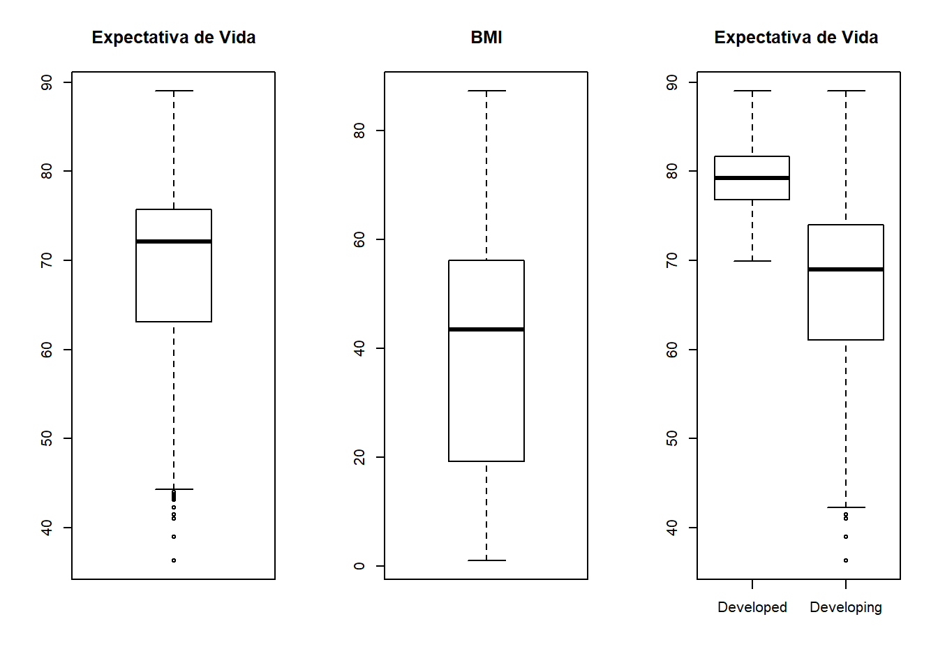
3.1.7 Examinando frequencia e distribuição dos dados
Você verá muito mais nas próximas aulas. Aqui nos deteremos a examinar apenas variáveis simples que informação sobre a frequencia e distribuição dos dados.
3.1.8 Frequência de valores
Não se preocupe com os gráficos agora. Você conhecerá mais sobre eles na próxima aula.
table(Cars93$Type)##
## Compact Large Midsize Small Sporty Van
## 16 11 22 21 14 9table(Cars93$Origin)##
## USA non-USA
## 48 45par(mfrow = c(1, 2))
barplot(table(Cars93$Type), main='Quantidade de Veículos por Tipo',col='orange')
barplot(table(Cars93$Origin), main='Quantidade de Veículos por Origem',col=c('green','blue'))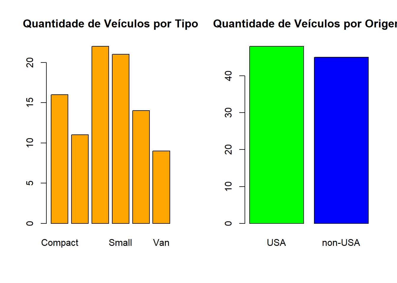
3.1.9 Estatísticas básicas
Mediana, Quartis, Variância, Desvio Padrão
summary(Cars93[ , c('Type','Make','Price','Cylinders','Horsepower')])## Type Make Price Cylinders Horsepower
## Compact:16 Acura Integra: 1 Min. : 7.40 3 : 3 Min. : 55.0
## Large :11 Acura Legend : 1 1st Qu.:12.20 4 :49 1st Qu.:103.0
## Midsize:22 Audi 100 : 1 Median :17.70 5 : 2 Median :140.0
## Small :21 Audi 90 : 1 Mean :19.51 6 :31 Mean :143.8
## Sporty :14 BMW 535i : 1 3rd Qu.:23.30 8 : 7 3rd Qu.:170.0
## Van : 9 Buick Century: 1 Max. :61.90 rotary: 1 Max. :300.0
## (Other) :87attach(Cars93)
median(Price)## [1] 17.7quantile(Horsepower)## 0% 25% 50% 75% 100%
## 55 103 140 170 300var(Price)## [1] 93.30458sd(Price)## [1] 9.65943# note
sqrt( var(Price) ) == sd(Price) ## [1] TRUEvar(Price) == sd(Price)**2## [1] TRUEpar(mfrow = c(1, 2))
boxplot(Price,main='Preços', col='yellow')
boxplot(Price ~ Type,data=Cars93,main="Preços por Tipo",col='lightBlue')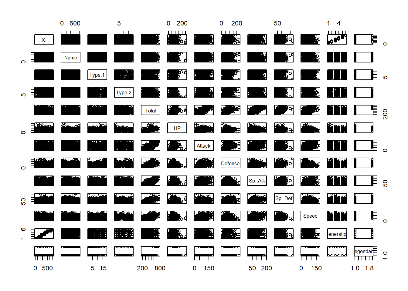
detach(Cars93)3.1.10 Distâncias inter quartis e remoção de Outliers
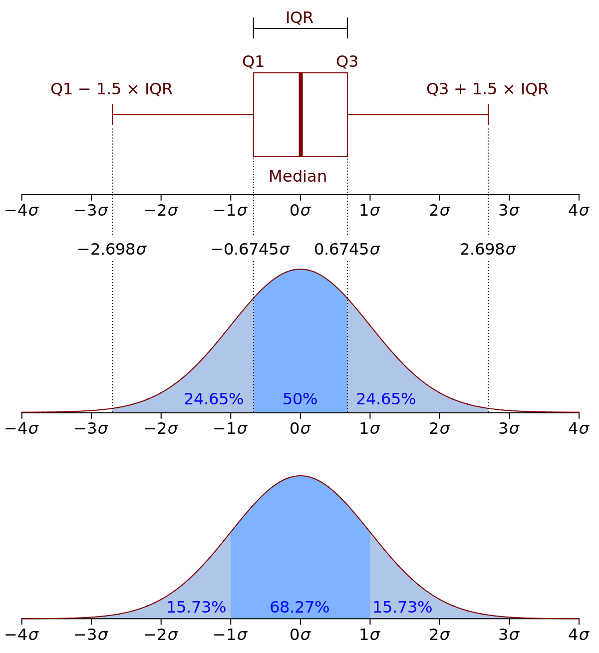
iqr = IQR(Cars93$Price); iqr## [1] 11.1Q = quantile(Cars93$Price, probs=c(.25, .75)); Q## 25% 75%
## 12.2 23.3up = Q[2]+1.5*iqr # Maior valor
low = Q[1]-1.5*iqr # Menor valor
head(Cars93[Cars93$Price > up,])## Manufacturer Model Type Min.Price Price Max.Price MPG.city MPG.highway
## 11 Cadillac Seville Midsize 37.5 40.1 42.7 16 25
## 48 Infiniti Q45 Midsize 45.4 47.9 50.4 17 22
## 59 Mercedes-Benz 300E Midsize 43.8 61.9 80.0 19 25
## AirBags DriveTrain Cylinders EngineSize Horsepower RPM
## 11 Driver & Passenger Front 8 4.6 295 6000
## 48 Driver only Rear 8 4.5 278 6000
## 59 Driver & Passenger Rear 6 3.2 217 5500
## Rev.per.mile Man.trans.avail Fuel.tank.capacity Passengers Length Wheelbase
## 11 1985 No 20.0 5 204 111
## 48 1955 No 22.5 5 200 113
## 59 2220 No 18.5 5 187 110
## Width Turn.circle Rear.seat.room Luggage.room Weight Origin
## 11 74 44 31 14 3935 USA
## 48 72 42 29 15 4000 non-USA
## 59 69 37 27 15 3525 non-USA
## Make
## 11 Cadillac Seville
## 48 Infiniti Q45
## 59 Mercedes-Benz 300Enrow(Cars93[Cars93$Price > up,])## [1] 3head(Cars93[Cars93$Price < low,])## [1] Manufacturer Model Type Min.Price
## [5] Price Max.Price MPG.city MPG.highway
## [9] AirBags DriveTrain Cylinders EngineSize
## [13] Horsepower RPM Rev.per.mile Man.trans.avail
## [17] Fuel.tank.capacity Passengers Length Wheelbase
## [21] Width Turn.circle Rear.seat.room Luggage.room
## [25] Weight Origin Make
## <0 rows> (or 0-length row.names)nrow(Cars93[Cars93$Price < low,])## [1] 0Identificamos então 3 valores apenas como outliers com valores acima do esperado. Veja as marcas (fabricantes) dos carros!!!
3.1.11 Covariância e Coeficiente de Determinação
Podem haver muitas relações entre duas variáveis. Um muito importante, entre valores numéricos é haver uma relação linear. Isso pode ser medido pela Covariância.
A covariância de duas variáveis \(x\) e \(y\) de um conjunto de dados mede como as duas estão linearmente relacionadas. Uma covariância positiva indicaria uma relação linear positiva entre as variáveis e uma covariância negativa indicaria o oposto.
A covariância da amostra é definida em termos dos meios da amostra como:
\[ s_{xy} = \frac{1}{n-1} \sum_{i}{n} (x_i - \bar{x})(y_i - \bar{y}) \] Da mesma forma, a covariância populacional é definida em termos da média populacional como:
\[ \sigma_{xy} = \frac{1}{n} \sum_{i}{n} (x_i - \mu_{x})(y_i - \mu_{y}) \] Note a semelhança com a variância de uma única variável.
O coeficiente de determinação permite analisar o quanto a relação é linear fornecendo um valor entre \([-1,1]\).
cov(Cars93$Price, Cars93$Horsepower)## [1] 398.7647cor(Cars93$Price, Cars93$Horsepower)## [1] 0.7882176Outras relações podem existir entre os dados e podemos examinar através de gráficos de pares de variáveis.
myCars = Cars93[ , c('Price',"MPG.city", 'Weight','Horsepower')]
pairs(myCars)
"MPG.city", 'Weight' parecem ter uma relação linear e, de fato, podemos calcular isso.
plot( Cars93[ , c("MPG.city", 'Weight')] )
cov(Cars93[ , c("MPG.city", 'Weight')])
## MPG.city Weight
## MPG.city 31.58228 -2795.095
## Weight -2795.09467 347977.893cor(Cars93[ , c("MPG.city", 'Weight')])## MPG.city Weight
## MPG.city 1.0000000 -0.8431385
## Weight -0.8431385 1.0000000abline(lsfit(Cars93$MPG.city, Cars93$Weight),col='red')
3.2 Exercícios
3.2.1 Exercício Resolvido
Considere a base.
df = read.csv('http://meusite.mackenzie.br/rogerio/TIC/mystocksn.csv')
head(df)
## data IBOV VALE3 PETR4 DOLAR
## 1 2020-01-02 118573 13.45 16.27 4.0163
## 2 2020-01-03 117707 13.29 15.99 4.0234
## 3 2020-01-06 116878 13.14 16.22 4.0570
## 4 2020-01-07 116662 13.23 16.06 4.0604
## 5 2020-01-08 116247 13.22 15.70 4.0662
## 6 2020-01-09 115947 12.99 15.75 4.0628Inspecione os dados. Quantos registros e quantidade de atributos, quais atributos, etc. Qual o valor mínimo e máximo do dólar neste período.
nrow(df)## [1] 43ncol(df)## [1] 5names(df)## [1] "data" "IBOV" "VALE3" "PETR4" "DOLAR"min(df$DOLAR)## [1] 4.0163max(df$DOLAR)## [1] 4.60623.2.2 Exercício
Forneça as principais estatísticas dos dados (média, median, quartis, variância, desvio padrão etc.) para os valores dos índices da base.
summary(df)## data IBOV VALE3 PETR4
## 2020-01-02: 1 Min. : 86067 Min. : 7.97 Min. : 7.26
## 2020-01-03: 1 1st Qu.:113766 1st Qu.:11.79 1st Qu.:14.21
## 2020-01-06: 1 Median :115528 Median :12.05 Median :14.63
## 2020-01-07: 1 Mean :113383 Mean :12.05 Mean :14.24
## 2020-01-08: 1 3rd Qu.:116689 3rd Qu.:13.19 3rd Qu.:14.91
## 2020-01-09: 1 Max. :119528 Max. :13.63 Max. :16.27
## (Other) :37
## DOLAR
## Min. :4.016
## 1st Qu.:4.164
## Median :4.242
## Mean :4.265
## 3rd Qu.:4.355
## Max. :4.606
## var(df[,-c(1)])## IBOV VALE3 PETR4 DOLAR
## IBOV 42519429.1351 7820.1173325 10475.7766396 -824.17369291
## VALE3 7820.1173 1.6568144 2.0101713 -0.18469124
## PETR4 10475.7766 2.0101713 2.8063904 -0.22750142
## DOLAR -824.1737 -0.1846912 -0.2275014 0.025067143.2.3 Exercício Resolvido
Faça um gráfico para exibir as relações de todos os pares de índice financeiros.
pairs(df[, -c(1)])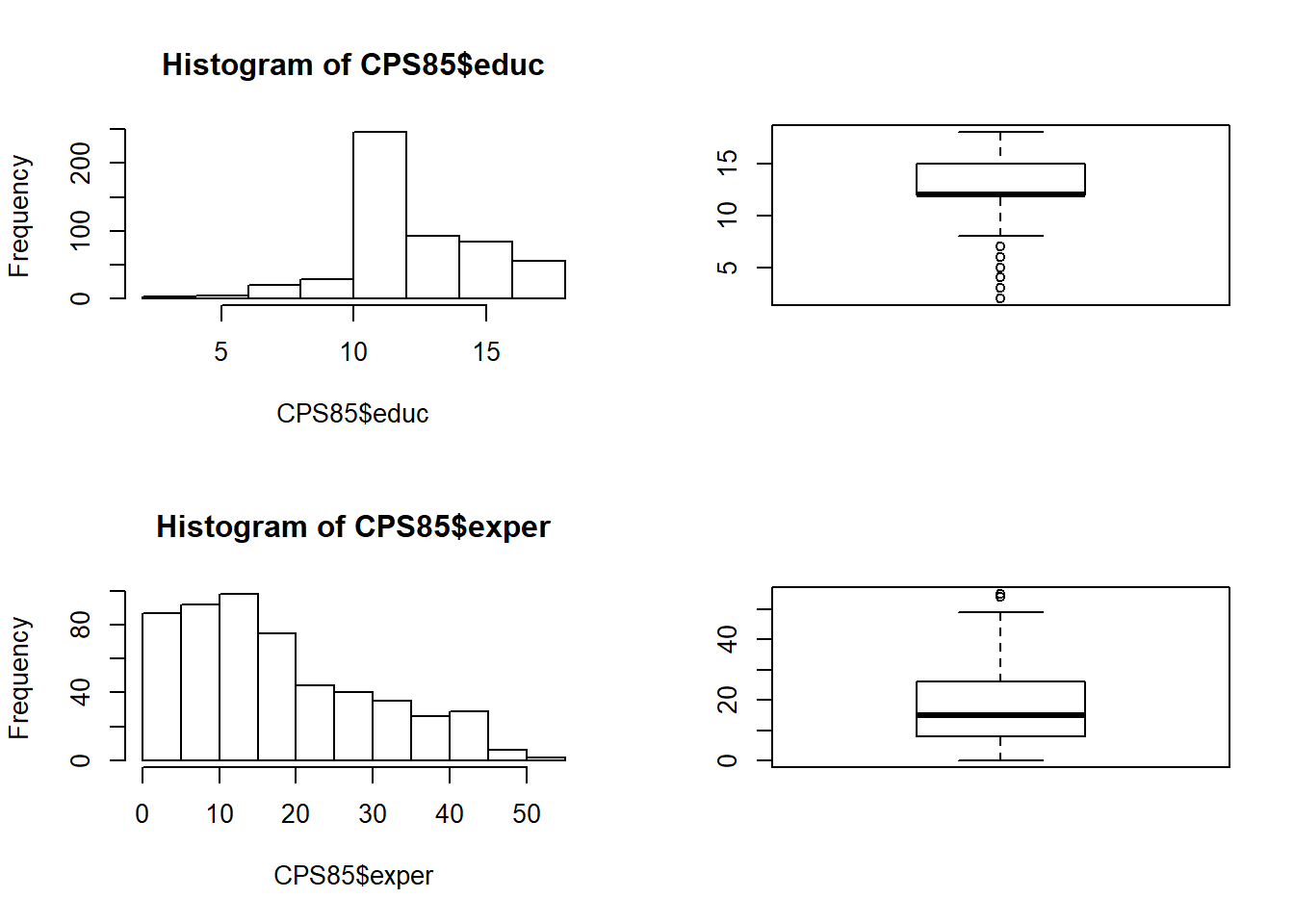
3.2.4 Exercício
Quais índices possuem um relação mais linear com o Dólar no período? (é preferível empregar o cor()).
cor(df$DOLAR,df[,-c(1)])## IBOV VALE3 PETR4 DOLAR
## [1,] -0.7983119 -0.9062686 -0.8577439 1cov(df$DOLAR,df[,-c(1)])## IBOV VALE3 PETR4 DOLAR
## [1,] -824.1737 -0.1846912 -0.2275014 0.025067143.2.5 Exercício Resolvido
Qual média de potência (Horsepower) dos veículos de Cars93 por origem?
for (t in unique(Cars93$Type)){
  cat(t , '\n',  str( mean(Cars93[Cars93$Type == t, ]$Price) ) )
}
## num 10.2
## Small
## num 27.2
## Midsize
## num 18.2
## Compact
## num 24.3
## Large
## num 19.4
## Sporty
## num 19.1
## Van3.2.6 Exercício
Considere a base.
df = read.csv('https://meusite.mackenzie.br/rogerio/TIC/Life_Expectancy_Data.csv')
df = na.omit(df)
head(df)
## Country Year Status Life.expectancy Adult.Mortality infant.deaths
## 1 Afghanistan 2015 Developing 65.0 263 62
## 2 Afghanistan 2014 Developing 59.9 271 64
## 3 Afghanistan 2013 Developing 59.9 268 66
## 4 Afghanistan 2012 Developing 59.5 272 69
## 5 Afghanistan 2011 Developing 59.2 275 71
## 6 Afghanistan 2010 Developing 58.8 279 74
## Alcohol percentage.expenditure Hepatitis.B Measles BMI under.five.deaths
## 1 0.01 71.279624 65 1154 19.1 83
## 2 0.01 73.523582 62 492 18.6 86
## 3 0.01 73.219243 64 430 18.1 89
## 4 0.01 78.184215 67 2787 17.6 93
## 5 0.01 7.097109 68 3013 17.2 97
## 6 0.01 79.679367 66 1989 16.7 102
## Polio Total.expenditure Diphtheria HIV.AIDS GDP Population
## 1 6 8.16 65 0.1 584.25921 33736494
## 2 58 8.18 62 0.1 612.69651 327582
## 3 62 8.13 64 0.1 631.74498 31731688
## 4 67 8.52 67 0.1 669.95900 3696958
## 5 68 7.87 68 0.1 63.53723 2978599
## 6 66 9.20 66 0.1 553.32894 2883167
## thinness..1.19.years thinness.5.9.years Income.composition.of.resources
## 1 17.2 17.3 0.479
## 2 17.5 17.5 0.476
## 3 17.7 17.7 0.470
## 4 17.9 18.0 0.463
## 5 18.2 18.2 0.454
## 6 18.4 18.4 0.448
## Schooling
## 1 10.1
## 2 10.0
## 3 9.9
## 4 9.8
## 5 9.5
## 6 9.2Qual a média de BMI e Expectativa de Vida para os países em desenvolvimento e desenvolvidos?
for (s in unique(df$Status)){
  cat(s , '\n',  str( mean(df[df$Status == s, ]$Life.expectancy) ) , '\n',  str( mean(df[df$Status == s, ]$BMI) ) )
}
## num 67.7
## num 35.7
## Developing
##
## num 78.7
## num 52.3
## Developed
## 3.2.7 Exercício
Existe correlação entre BMI e Expectativa de Vida para os desenvolvidos?
cor(df[df$Status == 'Developed', ]$Life.expectancy,df[df$Status == 'Developed', , ]$BMI) ## [1] 0.010794343.2.8 Exercício
Existem outliers de BMI e Expectativa de Vida no conjunto de todos os países?
par(mfrow = c(1, 2))
boxplot(df$Life.expectancy)
boxplot(df$BMI) 
print('Life.expectancy')## [1] "Life.expectancy"iqr = IQR(df$Life.expectancy); iqr## [1] 10.6Q = quantile(df$Life.expectancy, probs=c(.25, .75)); Q## 25% 75%
## 64.4 75.0up = Q[2]+1.5*iqr # Maior valor
low = Q[1]-1.5*iqr # Menor valor
df[df$Life.expectancy > up,]## [1] Country Year
## [3] Status Life.expectancy
## [5] Adult.Mortality infant.deaths
## [7] Alcohol percentage.expenditure
## [9] Hepatitis.B Measles
## [11] BMI under.five.deaths
## [13] Polio Total.expenditure
## [15] Diphtheria HIV.AIDS
## [17] GDP Population
## [19] thinness..1.19.years thinness.5.9.years
## [21] Income.composition.of.resources Schooling
## <0 rows> (or 0-length row.names)nrow(df[df$Life.expectancy > up,])## [1] 0df[df$Life.expectancy < low,]## Country Year Status Life.expectancy Adult.Mortality infant.deaths
## 57 Angola 2007 Developing 48.2 375 87
## 348 Botswana 2004 Developing 48.1 652 2
## 349 Botswana 2003 Developing 46.4 693 2
## 350 Botswana 2002 Developing 46.0 699 2
## 351 Botswana 2001 Developing 46.7 679 2
## 352 Botswana 2000 Developing 47.8 647 2
## 1482 Lesotho 2008 Developing 47.8 592 5
## 1483 Lesotho 2007 Developing 46.2 633 4
## 1484 Lesotho 2006 Developing 45.3 654 5
## 1485 Lesotho 2005 Developing 44.5 675 5
## 1486 Lesotho 2004 Developing 44.8 666 5
## 1487 Lesotho 2003 Developing 45.5 648 5
## 1579 Malawi 2007 Developing 48.5 559 37
## 1580 Malawi 2006 Developing 47.1 587 38
## 1581 Malawi 2005 Developing 46.0 66 39
## 1582 Malawi 2004 Developing 45.1 615 40
## 1583 Malawi 2003 Developing 44.6 613 43
## 1584 Malawi 2002 Developing 44.0 67 46
## 2299 Sierra Leone 2014 Developing 48.1 463 23
## 2303 Sierra Leone 2010 Developing 48.1 424 27
## 2304 Sierra Leone 2009 Developing 47.1 433 28
## 2305 Sierra Leone 2008 Developing 46.2 441 29
## 2306 Sierra Leone 2007 Developing 45.3 45 29
## 2499 Swaziland 2006 Developing 47.8 564 3
## 2500 Swaziland 2005 Developing 46.0 63 3
## 2501 Swaziland 2004 Developing 45.6 69 3
## 2502 Swaziland 2003 Developing 45.9 6 3
## 2503 Swaziland 2002 Developing 46.4 587 3
## 2504 Swaziland 2001 Developing 47.1 568 3
## 2505 Swaziland 2000 Developing 48.4 536 3
## 2930 Zimbabwe 2008 Developing 48.2 632 30
## 2931 Zimbabwe 2007 Developing 46.6 67 29
## 2932 Zimbabwe 2006 Developing 45.4 7 28
## 2933 Zimbabwe 2005 Developing 44.6 717 28
## 2934 Zimbabwe 2004 Developing 44.3 723 27
## 2935 Zimbabwe 2003 Developing 44.5 715 26
## 2936 Zimbabwe 2002 Developing 44.8 73 25
## 2937 Zimbabwe 2001 Developing 45.3 686 25
## 2938 Zimbabwe 2000 Developing 46.0 665 24
## Alcohol percentage.expenditure Hepatitis.B Measles BMI under.five.deaths
## 57 6.35 184.821345 73 1014 18.8 138
## 348 4.90 469.582390 91 1 32.2 4
## 349 5.51 299.367125 9 59 31.6 4
## 350 6.41 6.330007 88 7 31.1 4
## 351 5.48 306.952735 87 1 3.5 4
## 352 5.37 250.891648 86 2672 29.9 4
## 1482 2.75 91.854328 88 0 28.8 6
## 1483 2.69 9.184327 9 2 28.3 6
## 1484 2.61 71.155776 91 1 27.9 6
## 1485 2.67 57.903698 87 0 27.4 6
## 1486 1.80 67.913618 6 31 26.9 7
## 1487 1.99 5.300902 17 1 26.4 7
## 1579 1.18 4.269511 87 143 16.6 59
## 1580 1.18 6.847034 99 1 16.2 61
## 1581 1.04 5.670640 93 184 15.9 62
## 1582 1.11 58.135833 89 1116 15.5 65
## 1583 1.08 4.375316 84 167 15.2 70
## 1584 1.10 3.885395 64 92 14.8 75
## 2299 0.01 1.443286 83 1006 23.8 32
## 2303 3.84 5.347718 86 1089 21.7 40
## 2304 3.97 49.837127 84 31 21.2 42
## 2305 3.91 5.379606 77 44 2.7 44
## 2306 3.86 45.571089 63 0 2.2 45
## 2499 5.53 437.080244 93 0 28.2 4
## 2500 5.08 372.165147 95 0 27.8 4
## 2501 5.78 37.438577 93 0 27.4 4
## 2502 5.65 2.819124 9 350 27.1 4
## 2503 5.52 131.042127 88 37 26.7 4
## 2504 6.72 143.619732 86 49 26.3 4
## 2505 7.19 25.216833 83 10 25.9 4
## 2930 3.56 20.843429 75 0 28.6 46
## 2931 3.88 29.814566 72 242 28.2 46
## 2932 4.57 34.262169 68 212 27.9 45
## 2933 4.14 8.717409 65 420 27.5 43
## 2934 4.36 0.000000 68 31 27.1 42
## 2935 4.06 0.000000 7 998 26.7 41
## 2936 4.43 0.000000 73 304 26.3 40
## 2937 1.72 0.000000 76 529 25.9 39
## 2938 1.68 0.000000 79 1483 25.5 39
## Polio Total.expenditure Diphtheria HIV.AIDS GDP Population
## 57 75 3.38 73 2.6 2878.83714 2997687
## 348 96 5.56 96 28.4 4896.58384 182933
## 349 96 4.65 96 31.9 4163.65960 184339
## 350 97 6.47 97 34.6 355.61838 1779953
## 351 97 5.73 97 37.2 3128.97793 1754935
## 352 97 4.64 97 38.8 3349.68823 172834
## 1482 86 8.85 88 27.3 934.42856 199993
## 1483 87 8.47 88 30.0 918.43272 1982287
## 1484 88 7.12 89 34.1 915.77575 1965662
## 1485 88 6.30 89 34.8 862.94631 1949543
## 1486 89 6.96 9 34.6 781.51459 1933728
## 1487 9 7.13 9 33.8 63.63628 191897
## 1579 88 9.31 87 19.3 32.22273 1384969
## 1580 99 8.99 99 21.1 297.69712 13429262
## 1581 94 8.20 93 22.4 28.36738 1339711
## 1582 94 7.82 89 23.4 274.22563 1267638
## 1583 85 6.35 84 24.2 26.15252 12336687
## 1584 79 4.82 64 24.7 29.97990 1213711
## 2299 83 11.90 83 0.6 78.43948 779162
## 2303 84 1.32 86 1.6 45.12842 645872
## 2304 81 13.13 84 1.7 394.59324 63126
## 2305 75 1.29 77 1.9 46.37592 6165372
## 2306 63 1.12 64 2.2 358.82747 615417
## 2499 88 6.81 87 43.7 2937.36723 112514
## 2500 88 6.80 86 49.1 2873.86214 115873
## 2501 88 5.88 86 50.3 2529.63356 19553
## 2502 87 5.71 85 50.6 22.99449 187392
## 2503 87 5.16 85 49.9 1324.99623 1893
## 2504 87 5.11 84 48.8 1437.63495 172927
## 2505 87 5.26 84 46.4 1637.45670 161468
## 2930 75 4.96 75 20.5 325.67857 13558469
## 2931 73 4.47 73 23.7 396.99822 1332999
## 2932 71 5.12 7 26.8 414.79623 13124267
## 2933 69 6.44 68 30.3 444.76575 129432
## 2934 67 7.13 65 33.6 454.36665 12777511
## 2935 7 6.52 68 36.7 453.35116 12633897
## 2936 73 6.53 71 39.8 57.34834 125525
## 2937 76 6.16 75 42.1 548.58731 12366165
## 2938 78 7.10 78 43.5 547.35888 12222251
## thinness..1.19.years thinness.5.9.years Income.composition.of.resources
## 57 9.6 9.6 0.454
## 348 1.5 1.4 0.580
## 349 1.9 1.8 0.567
## 350 11.4 11.3 0.558
## 351 11.8 11.8 0.560
## 352 12.3 12.2 0.559
## 1482 8.0 7.8 0.447
## 1483 8.4 8.3 0.440
## 1484 8.8 8.7 0.437
## 1485 9.3 9.2 0.437
## 1486 9.7 9.7 0.439
## 1487 1.2 1.1 0.440
## 1579 7.1 7.0 0.387
## 1580 7.3 7.1 0.377
## 1581 7.4 7.2 0.371
## 1582 7.5 7.4 0.366
## 1583 7.6 7.5 0.362
## 1584 7.7 7.6 0.388
## 2299 7.5 7.4 0.426
## 2303 8.3 8.2 0.384
## 2304 8.5 8.4 0.375
## 2305 8.7 8.7 0.367
## 2306 8.9 8.9 0.357
## 2499 6.9 7.1 0.502
## 2500 7.3 7.5 0.495
## 2501 7.7 7.9 0.492
## 2502 8.2 8.4 0.493
## 2503 8.6 8.8 0.502
## 2504 9.0 9.2 0.506
## 2505 9.4 9.6 0.516
## 2930 7.8 7.8 0.421
## 2931 8.2 8.2 0.414
## 2932 8.6 8.6 0.408
## 2933 9.0 9.0 0.406
## 2934 9.4 9.4 0.407
## 2935 9.8 9.9 0.418
## 2936 1.2 1.3 0.427
## 2937 1.6 1.7 0.427
## 2938 11.0 11.2 0.434
## Schooling
## 57 7.7
## 348 11.8
## 349 11.8
## 350 11.9
## 351 11.8
## 352 11.7
## 1482 10.7
## 1483 10.6
## 1484 10.7
## 1485 10.7
## 1486 10.7
## 1487 10.5
## 1579 9.7
## 1580 9.6
## 1581 9.7
## 1582 10.0
## 1583 10.3
## 1584 10.4
## 2299 9.5
## 2303 8.7
## 2304 8.5
## 2305 8.3
## 2306 8.2
## 2499 9.9
## 2500 9.7
## 2501 9.4
## 2502 9.1
## 2503 9.2
## 2504 9.3
## 2505 9.4
## 2930 9.7
## 2931 9.6
## 2932 9.5
## 2933 9.3
## 2934 9.2
## 2935 9.5
## 2936 10.0
## 2937 9.8
## 2938 9.8nrow(df[df$Life.expectancy < low,])## [1] 39print('BMI')## [1] "BMI"iqr = IQR(df$BMI); iqr## [1] 36.3Q = quantile(df$BMI, probs=c(.25, .75)); Q## 25% 75%
## 19.5 55.8up = Q[2]+1.5*iqr # Maior valor
low = Q[1]-1.5*iqr # Menor valor
df[df$BMI > up,]## [1] Country Year
## [3] Status Life.expectancy
## [5] Adult.Mortality infant.deaths
## [7] Alcohol percentage.expenditure
## [9] Hepatitis.B Measles
## [11] BMI under.five.deaths
## [13] Polio Total.expenditure
## [15] Diphtheria HIV.AIDS
## [17] GDP Population
## [19] thinness..1.19.years thinness.5.9.years
## [21] Income.composition.of.resources Schooling
## <0 rows> (or 0-length row.names)nrow(df[df$BMI > up,])## [1] 0df[df$BMI < low,]## [1] Country Year
## [3] Status Life.expectancy
## [5] Adult.Mortality infant.deaths
## [7] Alcohol percentage.expenditure
## [9] Hepatitis.B Measles
## [11] BMI under.five.deaths
## [13] Polio Total.expenditure
## [15] Diphtheria HIV.AIDS
## [17] GDP Population
## [19] thinness..1.19.years thinness.5.9.years
## [21] Income.composition.of.resources Schooling
## <0 rows> (or 0-length row.names)nrow(df[df$BMI < low,])## [1] 03.2.9 Exercício
Qual a média de Expectativa de Vida com e sem outliers ?
print('Life.expectancy')## [1] "Life.expectancy"iqr = IQR(df$Life.expectancy); iqr## [1] 10.6Q = quantile(df$Life.expectancy, probs=c(.25, .75)); Q## 25% 75%
## 64.4 75.0up = Q[2]+1.5*iqr # Maior valor
low = Q[1]-1.5*iqr # Menor valor
head( df[df$Life.expectancy > up,] )## [1] Country Year
## [3] Status Life.expectancy
## [5] Adult.Mortality infant.deaths
## [7] Alcohol percentage.expenditure
## [9] Hepatitis.B Measles
## [11] BMI under.five.deaths
## [13] Polio Total.expenditure
## [15] Diphtheria HIV.AIDS
## [17] GDP Population
## [19] thinness..1.19.years thinness.5.9.years
## [21] Income.composition.of.resources Schooling
## <0 rows> (or 0-length row.names)nrow(df[df$Life.expectancy > up,])## [1] 0head( df[df$Life.expectancy < low,] )## Country Year Status Life.expectancy Adult.Mortality infant.deaths
## 57 Angola 2007 Developing 48.2 375 87
## 348 Botswana 2004 Developing 48.1 652 2
## 349 Botswana 2003 Developing 46.4 693 2
## 350 Botswana 2002 Developing 46.0 699 2
## 351 Botswana 2001 Developing 46.7 679 2
## 352 Botswana 2000 Developing 47.8 647 2
## Alcohol percentage.expenditure Hepatitis.B Measles BMI under.five.deaths
## 57 6.35 184.821345 73 1014 18.8 138
## 348 4.90 469.582390 91 1 32.2 4
## 349 5.51 299.367125 9 59 31.6 4
## 350 6.41 6.330007 88 7 31.1 4
## 351 5.48 306.952735 87 1 3.5 4
## 352 5.37 250.891648 86 2672 29.9 4
## Polio Total.expenditure Diphtheria HIV.AIDS GDP Population
## 57 75 3.38 73 2.6 2878.8371 2997687
## 348 96 5.56 96 28.4 4896.5838 182933
## 349 96 4.65 96 31.9 4163.6596 184339
## 350 97 6.47 97 34.6 355.6184 1779953
## 351 97 5.73 97 37.2 3128.9779 1754935
## 352 97 4.64 97 38.8 3349.6882 172834
## thinness..1.19.years thinness.5.9.years Income.composition.of.resources
## 57 9.6 9.6 0.454
## 348 1.5 1.4 0.580
## 349 1.9 1.8 0.567
## 350 11.4 11.3 0.558
## 351 11.8 11.8 0.560
## 352 12.3 12.2 0.559
## Schooling
## 57 7.7
## 348 11.8
## 349 11.8
## 350 11.9
## 351 11.8
## 352 11.7nrow(df[df$Life.expectancy < low,])## [1] 39df_noout = df[-(df$Life.expectancy < low),]
mean(df$Life.expectancy) ## [1] 69.3023mean(df_noout$Life.expectancy)## [1] 69.304923.2.10 Exercício
Considere a base.
library(MASS)
help(painters)
painters = na.omit(painters)
head(painters)
## Composition Drawing Colour Expression School
## Da Udine 10 8 16 3 A
## Da Vinci 15 16 4 14 A
## Del Piombo 8 13 16 7 A
## Del Sarto 12 16 9 8 A
## Fr. Penni 0 15 8 0 A
## Guilio Romano 15 16 4 14 AQuantos tipos de escolas de pintores existem? (unique ou table)
unique(painters$School)## [1] A B C D E F G H
## Levels: A B C D E F G Htable(painters$School)##
## A B C D E F G H
## 10 6 6 10 7 4 7 43.2.11 Exercício
A moda em estatística é valor mais frequente dos dados. Qual a moda das escolas de pintores?
table(painters$School)##
## A B C D E F G H
## 10 6 6 10 7 4 7 4Podemos ver que é 'D'.
3.2.12 Exercício Resolvido
Quantos pintores estão acima da média em composição?
painters[painters$Composition >= mean(painters$Composition), ]## Composition Drawing Colour Expression School
## Da Vinci 15 16 4 14 A
## Del Sarto 12 16 9 8 A
## Guilio Romano 15 16 4 14 A
## Perino del Vaga 15 16 7 6 A
## Raphael 17 18 12 18 A
## Fr. Salviata 13 15 8 8 B
## Primaticcio 15 14 7 10 B
## T. Zucarro 13 14 10 9 B
## Volterra 12 15 5 8 B
## Barocci 14 15 6 10 C
## Cortona 16 14 12 6 C
## L. Jordaens 13 12 9 6 C
## Vanius 15 15 12 13 C
## Palma Giovane 12 9 14 6 D
## Tintoretto 15 14 16 4 D
## Titian 12 15 18 6 D
## Veronese 15 10 16 3 D
## Albani 14 14 10 6 E
## Corregio 13 13 15 12 E
## Domenichino 15 17 9 17 E
## Guercino 18 10 10 4 E
## Lanfranco 14 13 10 5 E
## The Carraci 15 17 13 13 E
## Otho Venius 13 14 10 10 G
## Rembrandt 15 6 17 12 G
## Rubens 18 13 17 17 G
## Teniers 15 12 13 6 G
## Van Dyck 15 10 17 13 G
## Le Brun 16 16 8 16 H
## Le Suer 15 15 4 15 H
## Poussin 15 17 6 15 Hnrow(painters[painters$Composition >= mean(painters$Composition), ])## [1] 313.2.13 Exercício
Qual o pintor ou pintores com maior pontuação considerando todos os critérios? Não há muita surpresa aqui não?
painters['Score'] = painters[,c(1)] + painters[,c(2)] + painters[,c(3)] + painters[,c(4)]
head(painters)
## Composition Drawing Colour Expression School Score
## Da Udine 10 8 16 3 A 37
## Da Vinci 15 16 4 14 A 49
## Del Piombo 8 13 16 7 A 44
## Del Sarto 12 16 9 8 A 45
## Fr. Penni 0 15 8 0 A 23
## Guilio Romano 15 16 4 14 A 49painters[painters$Score == max(painters$Score), ]## Composition Drawing Colour Expression School Score
## Raphael 17 18 12 18 A 65
## Rubens 18 13 17 17 G 653.2.13.0.0.1 Exercício Resolvido
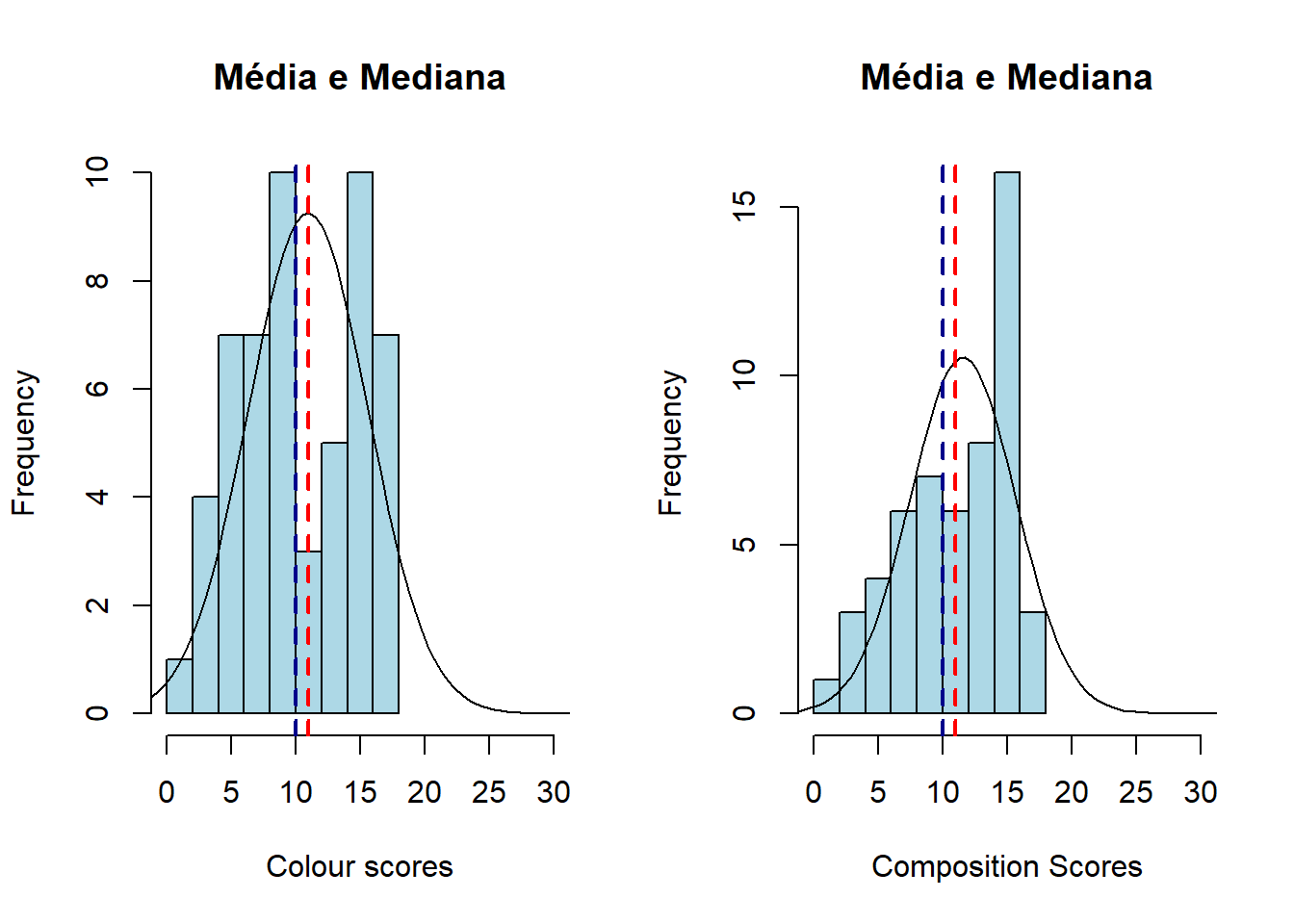
Mas esse nem é um ### Exercício (rs). Entenda a mediana e média através das notas de Composição e Colour dos pintores.
par(mfrow = c(1, 2))
x = painters$Colour
h = hist(x, col="lightblue", xlab="Colour scores", main="Média e Mediana", xlim=c(0,30))
xfit = seq(min(x)-3*sd(x),max(x)+4*sd(x),length=100)
yfit = dnorm(xfit,mean=mean(x),sd=sd(x))
yfit = yfit*diff(h$mids[1:2])*length(x)
lines(xfit, yfit, col="black", lwd=1)
abline(v=mean(painters$Colour),col='red',lty = 2, lwd = 2)
abline(v=median(painters$Colour),col='darkblue',lty = 2, lwd = 2)

x = painters$Composition
h = hist(x, col="lightblue", xlab="Composition Scores", main="Média e Mediana", xlim=c(0,30))
xfit = seq(min(x)-3*sd(x),max(x)+4*sd(x),length=100)
yfit = dnorm(xfit,mean=mean(x),sd=sd(x))
yfit = yfit*diff(h$mids[1:2])*length(x)
lines(xfit, yfit, col="black", lwd=1)
abline(v=mean(painters$Colour),col='red',lty = 2, lwd = 2)
abline(v=median(painters$Colour),col='darkblue',lty = 2, lwd = 2)